library(tidyverse)
library(ggplot2)
library(sf)
library(terra)
library(tidyterra)
library(rnaturalearth)
library(geodata)
library(sdmpredictors)

path<-"/home/data/spatial/" #this is a backup if we need to switch serversMaps & spatial data
Instructor: Riginos
Where on earth? Presenting and analysing spatial data using R
To undertake landscape genomics inherently requires working with spatial data. The individuals or populations that you have genotyped came from specific locations. It is likely that you will be interested in environmental attributes of that location. You might also want to calculate geographic distances between your sampling locations. And, undoubtedly you will want to plot your results on a map!
Spatial data, however, have their own unique issues and can be challenging to work with. This lesson is constructed as a basic introduction to working with spatial data and maps. If you understand the basics, then you can figure out how to do specific things that are relevant for your study.
At the end of this lesson, you will find a section on additional resources.
In this lesson you will:
- Become familiar with spatial data objects including points, lines, polygons, and rasters
- Obtain maps and manipulate them
- Start using coordinate reference systems
- Obtain and extract environmental information for georeferenced points
By the end of this lesson you should be able to:
- Create various spatial objects from xy coordinates and plot those objects
- Obtain appropriate distance measures between locations
- Assign an appropriate CRS to your spatial data object
- Plot and map spatial data against various map projections
- Import data from a biodiversity database
- Extract and summarize (terrestrial) environmental data for a series of points
Install packages and load libraries
In this lesson, we will focus on some common spatial data packages and will be using a controlled space. When you want to repeat these procedures on your own computer, you will need to install many packages. Some package dependencies can be tricky to install as they rely GDAL binaries (= other programs) on your computer. Try loading the package sf - if no errors are returned, you are good to go! If you do have errors try the instructions here.
#|echo: false

library(tidyverse)
library(ggplot2)
library(sf)
library(terra)
library(tidyterra)
library(rnaturalearth)
library(geodata)
library(sdmpredictors)

path<-"./home/data/spatial/" #this is a backup if we need to switch servers
Getting oriented with spatial data
Note: We will focus on spatial data structures as defined by packages sf and terra. sf stands for simple features is a newish package for vector data (points, lines, shapes: EPS is a common file format for vector data) that attempts to update older spatial tools (primarily from the package sp) but make formats and commands consistent with Tidyverse conventions and interfaces more readily with ggplot than the older sp.
Rasters are like picture images: the datasets are made up of equal sized cells, where each cell has a value and the smaller the cells, the more detailed the picture and the larger the file. JPGs and TIFs are raster formats, for example. Just as the above discussion on vector data, new packages are replacing old packages. We will use the new package, terra, that “plays well” with tidyverse and ggplot. Be aware, however, that many examples you find in the wild will have used the older raster package.
Examining and creating a simple features objects
To start getting familiar with spatial objects, we will download a simple map of Sweden from natural earth. Take a quick look at this website to get a sense of all the wonderful data that are available here. (You are welcome to make a map of any country you like).
#Extract information from natural earth
Sweden<- ne_countries(country = "sweden", returnclass = "sf")
plot(Sweden)
#Surprised? We will come back to this.

#Examine your new object
class(Sweden) #sf and data.frame
Sweden #tibble-like format!
Checking spatial data using plots (often) is highly recommended. You should also check the class of the object. The challenge question below shows you how to handle data that are imported incorrectly.
Challenge 1: Use subsetting commands to look at the first entry under the geometry column
Instead of the command you used above, try
Sweden2<- ne_countries(country = "sweden"). Usingclass()look at how the object is described and compare to your original object. What has happened is that rather than create an sf object, the older format of sp has been created. See if you can convertSweden2to the sf format using the functionst_as_sf().
Notice that spatial features objects take the form of a tibble. This means that all your standard Tidyverse commands will work just fine (selecting, filtering, etc).
You will also notice that there is information about a “bounding box” and “CRS” in your sf version of Sweden where in the sp version of Sweden2 you saw “extent” and “crs”. We will come back to that! Otherwise this object mostly looks like a normal tibble with lots of columns, but there is one special column, labelled geometry. You will notice that for Sweden the geometry is described as a “MULTIPOLYGON”… more on this in a moment too.
Challenge 2: Use subsetting commands to look at the first entry under the geometry column. Answers at end of this document, but you should be able to figure out these bits of code yourself! Try doing this using either base or tidy syntax, or both.
You should have an answer like this:
POLYGON ((11.02737 58.85615, 11.46827 59.43239, 12.30037 60.11793, 12.63115 61.29357, 11.99206 61.80036, 11.93057 63.12832……
Besides being an eyesore to look at, you might notice some patterns: the odd entries look a lot like longitude values and the even entries look like latitudes… because they are! This POLYGON is composed of a series of points that are connected to form the Swedish coastline.
We can get a better feeling for this with a simple example where we construct a series of simple features (this example is borrowed from the sf vignette). Try to understand what is going on with each bit of code.
## multipoints
p <- rbind(c(3.2,4), c(3,4.6), c(3.8,4.4), c(3.5,3.8), c(3.4,3.6), c(3.9,4.5))  #makes a matrix of x & y value
mp <- st_multipoint(p)  #defining p as multipoint object
plot(mp)  #you should see a series of points

## linestring
s1 <- rbind(c(0,3),c(0,4),c(1,5),c(2,5))
ls <- st_linestring(s1) # defining the linestring
plot(ls) #you should see a series of lines

## multilinestring
s2 <- rbind(c(0.2,3), c(0.2,4), c(1,4.8), c(2,4.8))
s3 <- rbind(c(0,4.4), c(0.6,5))
mls <- st_multilinestring(list(s1,s2,s3)) #notice the list function... #... applied to the matrices defining linestrings
plot(mls)

## multipolygon
p1 <- rbind(c(0,0), c(1,0), c(3,2), c(2,4), c(1,4), c(0,0))
pol1 <-st_polygon(list(p1))
plot(pol1)
p2 <- rbind(c(1,1), c(1,2), c(2,2), c(1,1))
pol2 <-st_polygon(list(p2))
plot(pol2)

## What happens if we combine polygons?
pol <-st_polygon(list(p1,p2))  #notice again the list function
plot(pol)  # do you see 2 polygons?
# The second polygon is a "hole" in the outer polygon!

## Now make it really messy!
p3 <- rbind(c(3,0), c(4,0), c(4,1), c(3,1), c(3,0))
p4 <- rbind(c(3.3,0.3), c(3.8,0.3), c(3.8,0.8), c(3.3,0.8), c(3.3,0.3))[5:1,]
p5 <- rbind(c(3,3), c(4,2), c(4,3), c(3,3))
# What do you think the following will look like?
# Test your predictions using plot()
mpol <- st_multipolygon(list(list(p1,p2), list(p3,p4), list(p5)))
Take a look again at your mpol object. As messy as this was to create, this is a pretty simple geometry and is captured by one MULTIPOLYGON entry. Go back now and look at mpol in its string form paying special attention to where the parentheses sit; their locations indicate if you have multiple polygons including holes within polygons.
Challenge 3: Make a grey square with a square hole in the middle.
Playing with some real spatial data
Only rarely do we need to manually create spatial feature. More likely we have data pre-packaged or we need to convert data. Use this link to download a csv file that has data for trees from the Bunya Mountains National Park in Queensland (one of my favorite places to go for a long weekend). These data come from my friend John Dwyer who is an awesome spatial ecologist (but is scared by genetics, sadly).
Import this csv file making sure to fix the path and file name to match your set up. Before you convert the dataframe to a spatial features object take at look at how it is structured. Repeat this after you convert it.
#load data
BunyaMountainTrees<-read_csv(paste0(path, "BunyaMountainTrees.csv"))

#Convert the tibble to a simple features object, with x and y coordinates
# Each row is a tree
BunyaMountainTrees<-st_as_sf(BunyaMountainTrees, coords = c("x", "y"))
What will plot(BunyaMountainTrees) look like? Surprised? (Does this remind you of what happened when you plotted Sweden?)
Try plot(BunyaMountainTrees, max.plot = 28). Although this might be confusing at first, this is really super cool… you are seeing the various column variables displayed in the appropriate location by individual tree. For now, we can concentrate on the species variable only. Try plot(BunyaMountainTrees["species"]). How cool is that! Let’s make this even better…
We will focus on ggplot solutions now, because the look nicer and are a bit easier.
ggplot(data = BunyaMountainTrees) +
        geom_sf(aes(col=species))
Challenge 4: Plot species identity for high-subplot 1, scaling the points by maximum tree diameter. Hint: Think about what units max_diam is in.
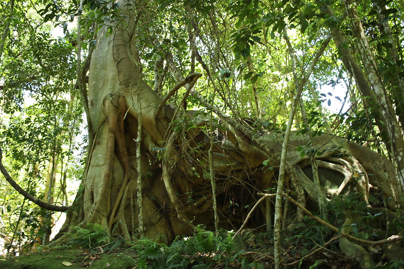
Notice which tree is the largest? It is a Ficus obliqua, the small leaf or strangler fig. Because they wrap around other trees and have buttressed roots, they can get quite wide around.
 Now that your data in in the sf format, there are many other things you can do. For example, you could examine the distance between all pairs of trees.
distances<-st_distance(BunyaMountainTrees, BunyaMountainTrees) #calculate distances, but this returns a symmetrical matrix

distances<-distances[lower.tri(distances)] #lower.tri returns T/F values...see if you can follow the subsetting being used here
ggplot(data = as.data.frame(distances)) +
  geom_histogram(mapping = aes(x = distances))
Keep in mind that the data are bounded by the size of the subplot. But it is interesting that you do not get too many trees very close together…why do you think that might be?
This function is very useful - for example you might want to calculate distances between your sampling locations to look for patterns of isolation by distance. When your data are in an x-y plane, st_distance will return the Euclidean distance. When your data are projected (see next section), then st_distance will calculate the distance on Earth’s sphere. Most of the commands in sf will automatically adjust when your data are spherical. But, it is worth occasionally checking and when you see very odd results, keeping in mind that an inappropriate distance measure could be being used.
Coordinate Reference Systems
Coordinate Reference Systems can cause major headaches and unexpected results if not handled properly. Make sure you understand the concepts in this section as it will save you time in the long run!
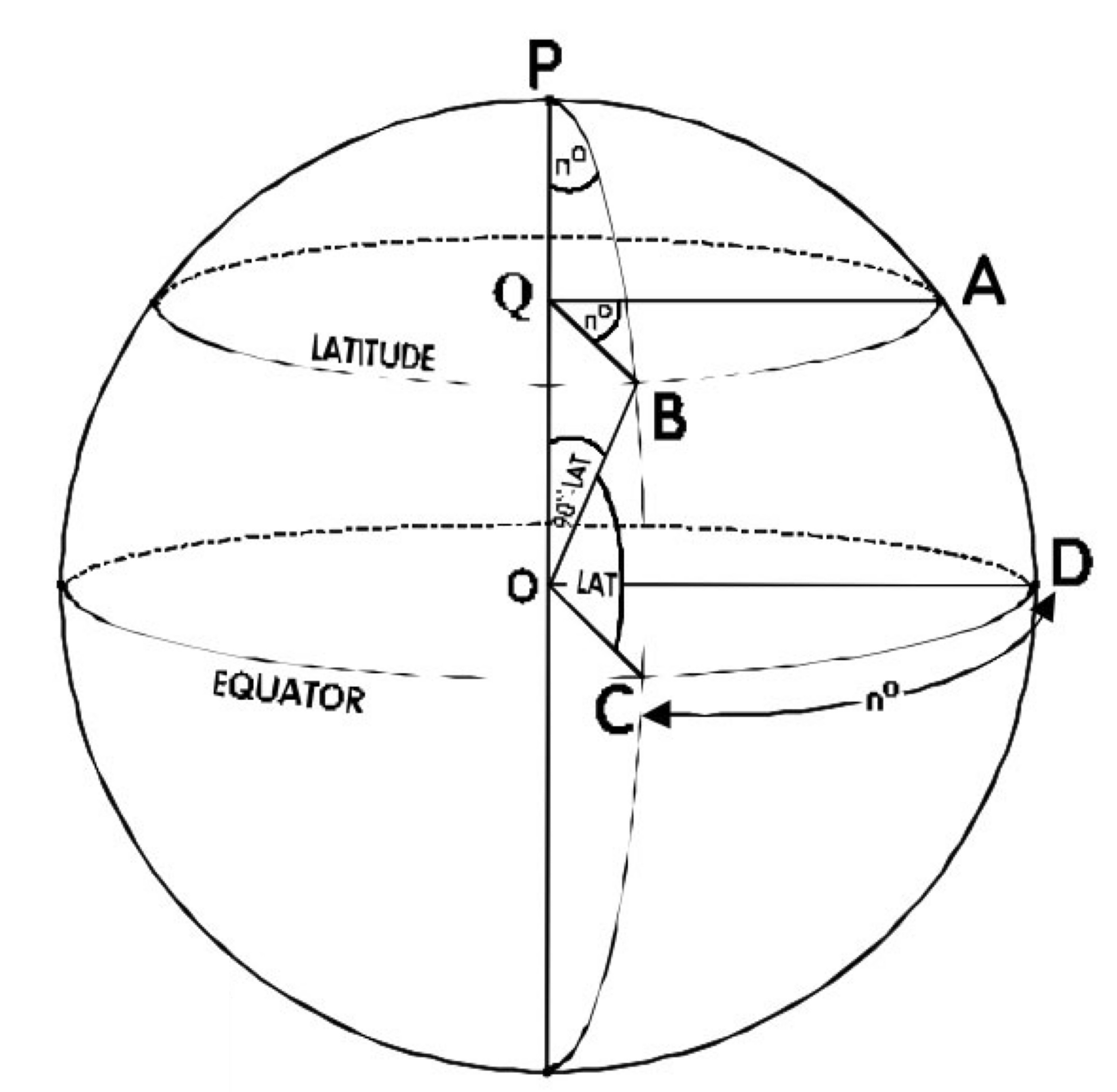
You are probably familiar with longitude and latitude as giving information about where on earth something is located. (Quick check: look up your own longitude and latitude based on your current location and where you were born.)
The problem with latitude is that if you compare two sets of points that sit on the same longitudes but at different latitudes, their distances will differ. The meridians (N-S lines on a globe) are farthest apart at the equator.
Projections involve taking the earth’s curvature into account are used to calculate relationships among spatial objects and to build 2D representative images. WGS 84 projection system is the most commonly encountered and works well for the whole earth scale. You can read more on WGS 84 in wikipedia. (Don’t worry if all this makes your head spin!)
To summarise:
- The earth is a sphere but we humans are used to thinking and projecting things in two dimensions. There is no universal (2D) projection system that preserves all relationships (distances, angles, areas) among a collection of points.
- There are many different projection systems that try to optimise certain relationships for specific locations on the earth. Conformal projections try to accurately show shapes but are inaccurate in sizes and distances (for example, Mercator Projection); equal-area projections preserve relative areas (for example, Lambert Equal Area or Mollweide); and equi-distant projections preserve distances (typically to a specific point on the map: see below).
- If you have two objects that you are trying to match up (say species occurences and temperature records) you need to make sure that they are in the same CRS.
- Depending on your analysis, especially if you need calculate areas (think about looking at species range areas, for example) you will need an equal area projection.
- The bigger the extent of your study region (like the whole earth, for example) the more these issues become important. At small scales they are less important.
Understanding and assigning Coordinate Reference Systems (CRS)
To start a deeper dive into CRS’s, go back to your now familiar Sweden object. Enter Sweden and also st_crs(Sweden).
Here we can see that the projection is longlat (= longitude and latitude), with datum (starting point, or 0 value) at WGS84 (= equator with longitude set at the prime meridian or Greenwich, UK).
We can also find the bounding box or extent of the spatial object, which represents the rectangular shape in which our map sits, where x & y positions are reported using decimal longitude and latitude. Try st_boundary(Sweden))
Note to your future self - longitude and latitude are very commonly reported incorrectly or in mixed formats. For example, rather than a decimal latitude of -38.2685, you might encounter 38° 16’ 6.6’’ S in degree-minute-second format. Or even worse you might get a mixture such as 38° 16.11’S ! Plot your data early on in any analysis to spot potential problems.
What about BunyaMountainTrees? Try to see what CRS is assigned….nothing! And actually given that we were just using x and y coordinates in meters, that’s fine. But, if we wanted to plot the data on a map we would have problems.
A file that accompanies BunyaMountainTrees is BunyaMountainSites. Import this and examine it. You might notice some funny variables called “easting” and “northing”; these are the positions of the plot sites in meters distant from a datum, a format called UTM or Universal Transverse Mercator. (A negative northing is in the southern direction.)
In order to attach the correct CRS details, however, we still need information on the projection…. Some further digging around on information provided by the authors gives us the following:
Location: Bunya Mountain National Park, Queensland Australia. Five areas of rainfortest or vine thicket were surveyed along a topographic moisture gradient: ‘high’ (easting = 359342, northing = 7027160) ‘low_east’ (365676, 7028551) ‘low_west’ (350888, 7030875) ‘mid_east’ (360196, 7027612) ‘mid_west’ (354971, 7031460) All eastings and northings in WGS84, zone 56.
Notice “WGS84, zone 56”. (Although N and S are not stated, we can guess that the projection is S since the Bunya Mountains are in the southern hemisphere!) Once you find the projection description, google it, and you will be likely directed to the relevant EPSG site. Here, we can use either the EPSG number or (scrolling down the page) copy the PROJ.4 text.
Here is how we assign the correct CRS to `BunyaMountainSites` and also turn it into an sf object.
BunyaMountainSites <-read_csv(paste0(path, "BunyaMountainSites.csv"))

BunyaMountainSites_sf<-st_as_sf(BunyaMountainSites, coords = c("easting", "northing"))  #convert the tibble to an sf object
st_crs(BunyaMountainSites_sf) <-"EPSG:32756"
#or
st_crs(BunyaMountainSites_sf) <-"+proj=utm +zone=56 +south +datum=WGS84 +units=m +no_defs"

#or we can convert and assign CRS in one step:
BunyaMountainSites_sf<-st_as_sf(BunyaMountainSites_sf, coords = c("easting", "northing"), crs="+proj=utm +zone=56 +south +datum=WGS84 +units=m +no_defs")
The website EPSG has lots of searchable information about CRS’s and projections; spend some time looking through their website. (Random trivia: EPSG stands for European Petroleum Survey Group. They created standards that have been widely adopted. EPSG is no longer associated with any industry group but the name persists.)
Transforming and reprojecting CRS’s
We have succeeded in adding a CRS to our BunyaMountainSites_sf object…but is it correct? A handy quick check would be to plot it on our map of Australia. How can we do this? First, import a map of Australia as you did earlier for Sweden and use the st_crs() function to look at the CRS’s of each object…are they the same?
To convert the CRS of bunya_sites_sf to match Australia is quite straightforward using the st_transform() function that undertakes a lot of serious geometric calculations for us. We can do this a number of ways:
# import map of Australia from natural earth
Australia<- ne_countries(country = "australia", returnclass = "sf")
st_crs(Australia)

# transform CRS
BunyaMountainSites.wgs84<-st_transform(BunyaMountainSites_sf, crs=4326)
#or
BunyaMountainSites.wgs84<-st_transform(BunyaMountainSites_sf, crs="+proj=longlat +datum=WGS84 +no_defs +ellps=WGS84 +towgs84=0,0,0")
#or
BunyaMountainSites.wgs84<-st_transform(BunyaMountainSites_sf, st_crs(Australia))
#All of these methods are equivalent
Now to plot these points on the map…
ggplot(data = Australia) +
  geom_sf() +  #background map needs to be first argument
  geom_sf(data = BunyaMountainSites.wgs84, size = 4, shape = 23, fill = "darkred") #our sites plotted on top
Why have I had you play around with this dataset on Australian trees? Because this dataset presents some of the irregularities and problems you might face when finding spatial data. You will often have to do some detective work and guessing to find and assign the correct CRS. Always test by plotting your data!
Consider three commonly used but different CRS’s:
- EPSG: 4326 = WGS84. For the whole earth, used by most GPS’s and Google Earth. Not equal area and technically not really projected. This one is an all-around compromise. It is centered on the equator and prime meridian
- EPSG:3006 = SWEREF99: This is for all of Sweden. It is a conformal projection that attempts to make both distances and area well represented. Good for making Swedish maps and Swedish focused analyses.
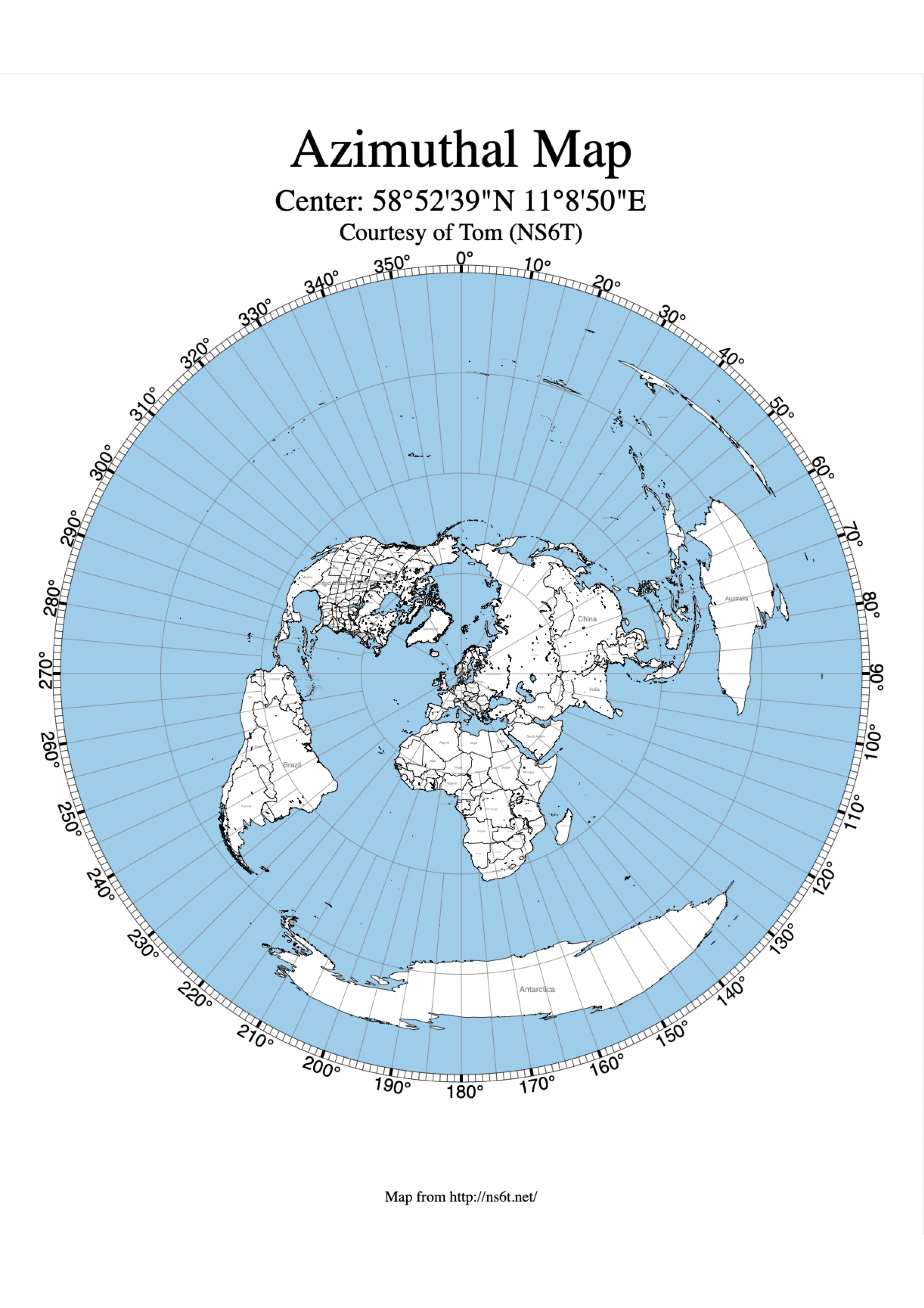
- Lambert Equal Area Azimuthal = LAEA: equal area projection and can be centered where we choose.
Our data is already in WGS84 but if we needed to define it the code would be:
WGS<-"+proj=longlat +datum=WGS84 +no_defs"
The code for SWEREF99 is: SWEREF99 <- "+proj=utm +zone=33 +ellps=GRS80 +towgs84=0,0,0,0,0,0,0 +units=m +no_defs +type=crs"
And for LAEA centered on the WGS84 datum: LAEA <- "+proj=laea +lat_0=0 +lon_0=0" (to center in Sweden: laea <- "+proj=laea +lat_0=16.321998712 +lon_0=62.38583179")
To see what those different projections look like, we can got back to our map of Sweden. We can reproject the CRS as follows:
WGS<-"+proj=longlat +datum=WGS84 +no_defs"

SWEREF99 <- "+proj=utm +zone=33 +ellps=GRS80 +towgs84=0,0,0,0,0,0,0 +units=m +no_defs +type=crs"

LAEA <- "+proj=laea  +lat_0=16.321998712 +lon_0=62.38583179"

Sweden.SWEREF99 <-st_transform(Sweden, SWEREF99)
Sweden.LAEA<-st_transform(Sweden, LAEA)
Challenge 5: Plot your original Sweden WGS and two reprojected maps. Then, change the LAEA projection to be centred on the prime meridien and plot that map again.
Note to your future self: Make sure that CRS are the same between objects that you are seeking to compare and map. It is easy to get caught out.
Add example of reading in river data
Raster data
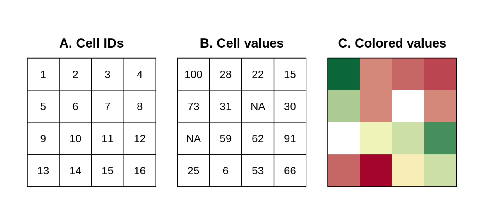
Points, lines, and polygon are vector objects: only a few points need to be specified to define them. In contrast, rasters are like picture images: each cell has a value and the smaller the cells, the more detailed the picture and the larger the file. Rasters are rectangular in shape and cells are ordered by row, whereby each cell can have a continuous or categorical value:
To start exploring rasters, we are going download information on world topography (altitude). One the most widely used sources of weather data come from WorldClim.org - these include historical and projected future climate data. They are especially useful for people working on terrestrial species and can be accessed using the library(geodata). Elevation (altitude is also included).
We can download elevation information for Sweden quite easily:
#This will take a few minutes to load.
elevation<- elevation_30s(country="Sweden", path=tempdir() )
ggplot() +
geom_raster(data = elevation, aes(x = x, y = y, fill = SWE_elv_msk), show.legend = FALSE) +
scale_fill_gradient(low = "lightgray", high = "black") +
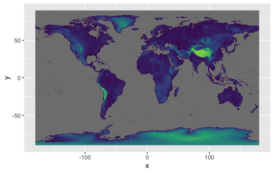
theme_void()In mid October the worldclim server was down for maintenance, so we will also explore a marine example. This example will extract Sea Surface Temperature (SST) from bio-ORACLE
SST <- load_layers("BO_sstmax")
SST<-terra::rast(SST) #now is terra compatible


ggplot() +
  geom_spatraster(data = SST)
Which ever raster you have downloaded, examine the structure by calling the name, using summary() and any other tools you like. Do you see some similarity in structure to sf objects? All of these spatial objects include an extent (= maximum and minimal locations, sometimes called the bounding box) and CRS. Notice that the raster additionally includes information on dimensions and resolution. Sometimes the units can be a bit mysterious and may need to do some investigation to understand them.
Cropping a raster
Rasters can be manipulated in manners similar to sf objects. In the example that follows, we are going to crop the global SST data to match the spatial extent of our Sweden vector object.
#first check that both objects have the same crs
same.crs(Sweden, SST)

# crop based on the spatial extent of Sweden
SST.sw<-terra::crop(SST, Sweden)

# plot to check
ggplot() +
  geom_spatraster(data = SST.sw)
Obviously that crop is a bit too close. There are many solutions for how to do this, but I will show you a manual solution so you can understand the spatialExtent or bounding box of an spatial object.
#diagnose the problem - look at the "bounding box" for the vector object
st_bbox(Sweden)

# and look at the "extent" for the raster
ext(SST.sw)

#Rounding error has resulted in ugliness!

#manually set the extent to crop
SST.sw<-terra::crop(SST, c(4, 24, 55, 70))

# plot to check
ggplot() +
  geom_spatraster(data = SST.sw)
Reprojecting a raster
Like vector data, rasters can be reprojected. Try the following code to project SST.sw to the LAEA0 projection. Then plot it.
LAEA0 <- "+proj=laea  +lat_0=0 +lon_0=0"

# raster reprojection
SST.sw.laea<-project(SST.sw, LAEA0)
Surprised?
Each time you reproject, however, you alter your raster. Therefore you should try to avoid doing this too much and it is generally best practice to reproject your vector data to match your raster’s CRS. (You can reproject vector objects back and forth endlessly without loosing information…why?)
General tips in working with rasters
- Use a coarse granularity of data to optimise your code and plotting and then for the final analyses (and graphics) use the finer resolution.
- Reproject once only.
- Project before cropping.
Finding suitable environmental data layers
A major challenge for any land/river/seascape analyses is finding appropriate environmental layers. Pre-compiled sources such as such as worldclim and bio-ORACLE are certainly popular. (Look at Hydrosheds for freshwater data). However, these ready to use packages might not be appropriate to your question and scale. The reality is that you will have to search for appropriate data sources and figure out how to import them, project them, etc. Often government agencies will have useful regional datasets. Each project is different and will involve its own challenges!
Compilations of possible environmental data sources
Terrestrial focused
- Leempoel, K., Duruz, S., Rochat, E., Widmer, I., Orozco-terWengel, P., & Joost, S. (2017). Simple rules for an efficient use of geographic information systems in molecular ecology. Frontiers in Ecology and Evolution, 5. doi:10.3389/fevo.2017.00033 Table 1 and Appendix
Marine focused
- Riginos, C., Crandall, E. D., Liggins, L., Bongaerts, P., & Treml, E. A. (2016). Navigating the currents of seascape genomics: how spatial analyses can augment population genomic studies. Current Zoology, 62(6), 581-601. doi:papers3://publication/doi/10.1093/cz/zow067 Table 1
Aquatic (marine and freshwater)
Selkoe, K. A., Scribner, K. T., & Galindo, H. M. (2016). Waterscape genetics – applications of landscape genetics to rivers, lakes, and seas. In N. Balkenhol, S. A. Cushman, A. Storfer, & L. P. Waits (Eds.), Landscape Genetics: Concepts, Methods, Applications (pp. 1-27): John Wiley & Sons, Ltd. Box 13.1
Grummer, J. A., Beheregaray, L. B., Bernatchez, L., Hand, B. K., Luikart, G., Narum, S. R., & Taylor, E. B. (2019). Aquatic landscape genomics and environmental effects on genetic variation. Trends in Ecology and Evolution, 1-14. doi:10.1016/j.tree.2019.02.013 Table 2
Further resources
Working with spatial data generally
Fantastic and comprehensive entry level open source book. Geocomputation with R
General explanations on using R for biological spatial data including remote sensing rspatial.org
A series of well explained tutorials for making publication-ready maps:
Another open source book: Spatial Data Science
Specific R package support
sf package vignettes - these are rather technical
marmap package with excellent vignettes - an essential resource if using marine data that allows you to draw bathymetric maps
Answers to challenge questions
Challenge 1
Use subsetting commands to look at the first entry under the geometry column
Sweden2<- ne_countries(country = "sweden")  #extracts information from natural earth
class(Sweden2)  #note that this is a SpatialPolygonsDataFrame... this is an sp object, but we want an sf object
Sweden2  #take a peak at the structure of this class object
Sweden2 <-st_as_sf(Sweden2 ) #convert to an sf object
class(Sweden2 ) #sf and data.frame
Sweden2  #tibble-like format!
Challenge 2
Use subsetting commands to look at the first entry under the geometry column
#Base solution
Sweden[[1,"geometry"]]

#Tidy solution
Sweden %>%
  filter(row_number() == 1) %>%
  select(geometry)
Challenge 3
Make a grey square with a square hole in the middle.
p_outer <- rbind(c(0,0), c(1,0), c(1,1), c(0,1), c(0,0))
p_inner<- rbind(c(0.25,0.25), c(0.75,0.25), c(0.75,0.75), c(0.25,0.75), c(0.25,0.25))

square <- st_multipolygon(list(list(p_outer,p_inner)))
plot(square, col="grey")
What happens if you use square <- st_multipolygon(list(list(p_outer), list(p_inner)))? Why?
Challenge 4
Plot species identity for high-subplot 1, scaling the points by maximum tree diameter.
ggplot(BunyaMountainTrees) +
     geom_sf(aes(col=species, size= max_diam))
Challenge 5
Plot your original Sweden WGS and two reprojected maps. Then, change the LAEA projection to be centred on the prime meridien and plot that map again.
# plotting reprojections

ggplot(data = Sweden.SWEREF99) +
    geom_sf()

ggplot(data = Sweden.LAEA) +
    geom_sf()

#LAEA centered on 0,0
LAEA0 <- "+proj=laea  +lat_0=0 +lon_0=0"
Sweden.LAEA0<-st_transform(Sweden, LAEA0)

ggplot(data = Sweden.LAEA0) +
    geom_sf()
#Not as good as centering on the country. Try Australia with LAEA0 if you want to see something truly awful.